[파이토치] RNN

Recurrent Neural Networks

• As you are reading the present sentence, you are processing it word by word while keeping memories of what came before.
• A recurrent neural network (RNN) processes sequences by iterating through the sequence elements and maintaining a state containing information relative to what it has seen so far.
  • The network internally loops over sequence elements.

 

scaler = MinMaxScaler()
df[['Open','High','Low','Close','Volume']] = scaler.fit_transform(df[['Open','High','Low','Close','Volume']])

# CPU/GPU

device = torch.device("cuda:0" if torch.cuda.is_available() else "cpu")

print(f'{device} is available.')

# Dataset

X = df[['Open','High','Low','Volume']].values

y = df['Close'].values

# Sequence를 생성하는 함수
def seq_data(x, y, sequence_length):

    

    x_seq = []

    y_seq = []

    for i in range(len(x)-sequence_length):

        x_seq.append(x[i:i+sequence_length]) # a[2:6] -> 2,3,4,5

        y_seq.append(y[i+sequence_length]) # 지난 5일을 통해서 다음날의 종가를 구한다.

    

    return torch.FloatTensor(x_seq).to(device), torch.FloatTensor(y_seq).to(device).view([-1, 1]) 

split = 200

sequence_length = 5

x_seq, y_seq = seq_data(X, y, sequence_length)

x_train_seq = x_seq[:split]

y_train_seq = y_seq[:split]

x_test_seq = x_seq[split:]

y_test_seq = y_seq[split:]

print(x_train_seq.size(), y_train_seq.size())

print(x_test_seq.size(), y_test_seq.size())

train = torch.utils.data.TensorDataset(x_train_seq, y_train_seq)

test = torch.utils.data.TensorDataset(x_test_seq, y_test_seq)

batch_size = 20

train_loader = torch.utils.data.DataLoader(dataset=train, batch_size=batch_size, shuffle=False)

test_loader = torch.utils.data.DataLoader(dataset=test, batch_size=batch_size, shuffle=False)

 

# RNN hyper-parameter
input_size = x_seq.size(2)
num_layers = 2 # 크기가 과도하게 클경우 overfitting 가능성이 커짐
hidden_size = 8 # 크기가 과도하게 클경우 overfitting 가능성이 커짐

 

class VanillaRNN(nn.Module):    

    def __init__(self, input_size, hidden_size, sequence_length, num_layers, device):

        super(VanillaRNN, self).__init__()

        self.device =device

        self.hidden_size = hidden_size

        self.num_layers = num_layers

        self.rnn = nn.RNN(input_size, hidden_size, num_layers, batch_first=True) # pytorch에서 제공하는 RNN은 sequence length가 먼저 들어와야하는데, batch_size가 첫번째로 들어왔다. 따라서 순서를 바꾸어하므로, batch_first=True로 선언한다. 

        self.fc = nn.Sequential(nn.Linear(hidden_size*sequence_length, 1), nn.Sigmoid())

        

    def forward(self, x):

        h0 = torch.zeros(self.num_layers, x.size()[0], self.hidden_size).to(self.device) # 초기 hidden state 설정

        out, _ = self.rnn(x, h0) # out: RNN의 마지막 레이어로 부터 나온 output feature 반환, hn: hidden state 반환

        out = out.reshape(out.shape[0], -1) # many to many 전략. 각각의 일자에 대해서 output도출한다.

        out = self.fc(out)

        return out

model = VanillaRNN(input_size=input_size, 

                   hidden_size=hidden_size, 

                   sequence_length=sequence_length, 

                   num_layers=num_layers, 

                   device=device).to(device)

criterion = nn.MSELoss()

lr = 1e-3

num_epochs = 200 

optimizer = optim.Adam(model.parameters(), lr=lr)

loss_graph = []

n = len(train_loader)

for epoch in range(num_epochs):

    running_loss = 0.0

    

    for data in train_loader:

        

        seq, target = data # 배치 데이터 

        out = model(seq)

        loss = criterion(out, target)

        

        optimizer.zero_grad()

        loss.backward()

        optimizer.step()

        running_loss += loss.item()

    

    loss_graph.append(running_loss/n)

    if epoch % 100 == 0:

        print('[epoch: %d] loss: %.4f' %(epoch, running_loss/n))

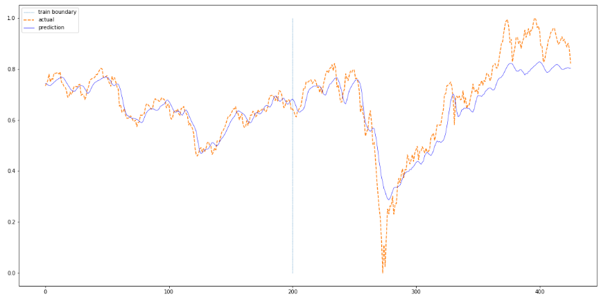
# 실제값과 예측값 비교
def plotting(train_loader, test_loader, actual):

    with torch.no_grad():

        train_pred = []

        test_pred = []

   

        for data in train_loader:

            seq, target = data # 배치 데이터 

            #print(seq.size())

            out = model(seq)

            train_pred += out.cpu().numpy().tolist()

            

        for data in test_loader:

            seq, target = data # 배치 데이터 

            #print(seq.size())

            out = model(seq)

            test_pred += out.cpu().numpy().tolist()

    total = train_pred+test_pred       

    plt.figure(figsize=(20,10))

    plt.plot(np.ones(100)*len(train_pred),np.linspace(0,1,100),'--', linewidth=0.6)

    plt.plot(actual,'--')

    plt.plot(total,'b', linewidth=0.6)

    

    

    plt.legend(['train boundary','actual','prediction'])

    plt.show() 

    

plotting(train_loader, test_loader, df['Close'][sequence_length:].values)        

실제 주가와 예측 주가의 비교 그래프